
MMT founders Warren Mosler and Randall Wray like to claim that ‘monetary policy has it backwards’, see these 1,5 min video quotes:
To offer some more detailed explanation of why I do not subscribe to W. Mosler‘s claim, I‘ll sketch another, imho more coherent view of how interest rate policy ‚transmits‘ to the price level of consumer goods that‘s pretty ‚Keynesian‘ to me (and not Moslerian at all), but also goes beyond Keynes in one important aspect by identifying a core implicit general assumption Keynes made, and specifying the situations where this assumption actually applies – and those situations where it does NOT apply.
The short answer to the questions raised in the title of this article would be: (1) MMT and the Money View both fail to conceptualize how interest rate policy translates to the price level of nonfinancial assets because they fail to conceptualize the relation & interactions between the ‘real’ and ‘financial’ spheres precisely enough. (2) One key to conceptualize this more clearly is the category of net financial assets and the balances of payments systematic of national accounting (rather than Morris Copeland’s flow of funds accounts). (3) A second conceptual key is the systematic distinction between ex post accounting categories and ex ante accounting categories: actually achieved flows vs. desired/planned flows.
But, let’s move into the details step by step.
The overall view I will sketch here is based on my reading/interpretation of Wolfgang Stützel‘s work mainly from the 1950s-1980s, which like MMT is also based on an ex post sectoral accounting framework (i.e. an accounting/balance sheet based circuit model of a closed economy). Stützel imports Keynes‘ core GT ideas on employment, interest and money into the sectoral accounting framework, but specifies and clarifies them by additional distinctions. He also provides a realistic systematic microfoundation in business practice that is very similar to Perry Mehrling’s dealer model, but applies to non-financial corporations as well and also systematically connects to a ‘sectoral accounting’ monetary circuit model of a closed economy (as a simple example for this, see his micro-absorption approach of explaining current account balances of small countries, also linked at the end of this text).
Unfortunately, no english translation of this particular – core – part of Stützel‘s work exists yet. We did very shortly present it at our 2017 seminar at BI Norwegian Business School, which had focused more on our overall legal institutionalist framework and its connection to macro accounting. The seminar talks & presentations are linked at the end of this text.
Here, I‘ll try to be as brief as possible, hoping it will still be accessible.
Wolfgang Stützel (1925-1987), was a very influential post war german economist (see this tribute volume published in 2001). He grew up in an entrepreneurial home: his father had a business producing pottery. Following his 1952 dissertation on ‘price, value and power’, Stützel worked at Berliner Bank from 1953-1957, followed in January 1957 by working for the Bank Deutscher Länder, which in August 1957 became Deutsche Bundesbank, until August 1958. During this time, he produced his foundational works, importing the power theory of value developed in his 1952 dissertation into a monetary circuit model of a closed economy based on balance sheets: the ‘Paradoxa der Geld und Konkurrenzwirtschaft’ (1953; published only in 1979) and the ‘Volkswirtschaftliche Saldenmechanik’ (1958). This approach was common at the time (Morris Copeland had published his ‘A Study of Moneyflows in the U.S.’ in 1952); however, Stützel imported some crucial specifications from business accounting practice into the model and introduced a core macro concept he called ‘lockstep’, which we will only cover in passing in this article (see Prof. Johannes Schmidt’s presentation and paper , which can also be found in the Journal of the History of Economic Thought, Vol. 26, 2019, Issue 6, pp. 1310-1340). In 1959, Stützel became a Professor of Economics at University of Saarland, teaching business administration, banking management and economics with a focus on money, currency and credit. He seeked a close cooperation with the Law faculty, suggesting an Institute for Civilistic Studies.
From 1966-1968, he was part of the german council of economic experts (‘Sachverständigenrat zur Begutachtung der gesamtwirtschaftlichen Entwicklung’) advising the german government in economic questions in the 1960s, and produced a number of theoretical innovations, such as his micro absorption theory to explain balances on current account. Nevertheless, his foundational texts, his 1952 Dissertation (‘Price, Value and Power – Analytical Theory of the Economy’s relation to the State’) and a major 1953 followup text importing the power theory of value developed there into a sectoral accounting framework (‘Paradoxes within Monetary Economies’) never got read or discussed much as they were published in book form only more than 20 years later, in 1972 and 1979.
Reading texts by MMTers, specifically Wray, and studying Perry Mehrling’s Money and Banking course had helped to prepare me for studying Stützels often difficult work, but as I did, I found that in a number of significant points, Stützel had achieved what I consider significant additional clarifications beyond MMT (and other post keynesian monetary circuit models) as early as the 1950s (the postwar ‘Keynesian’ era MMT also draws upon).
For the following, I will presuppose you know and understand the standard MMT ex post sectoral accounting framework where all financial assets always net to zero with their corresponding financial liabilities, and where there is a clear awareness of how different transactions lead to different types of quadruple entry balance sheet changes. This will be neccessary to understand the argument.
So: a raise in central bank interest rates would raise yields/period on financial assets and costs on financial liabilities. But this would also immediately reduce the current price of those already existing financial assets the central bank offers to buy & monetize, as the series of future payments these assets entitle to would need to be discounted with a now higher market interest rate. This would lead to a direct reductions in net worth of the holders of those assets. If financial institutions‘ net worth in relation to their financial assets is very low anyway, a drastic raise in interest rates – no matter if induced by private market actors or the central bank as a private market actor with a public mandate – can directly lead to insolvencies of financial firms, even to the point of chain insolvencies of banks and bank runs like we saw in 1931. Thus, an important post 2008 reform effort was to raise capital requirements (net worth to total assets ratio) for financial institutions.
Short disgression: I’d strongly recommend Perry Mehrling‘s money & banking course on that topic, but in this short blog entry, I don‘t want to focus on what interest rate policy means for the financial sector, which Perry Mehrling exclusively focuses on, but on what it means for the nonfinancial sector (nonfinancial firms, i.e. firms producing nonfinancial products/assets & services) from one particular perspective, focussing on one particular ‚transmission‘ from the financial to the ‚real‘ sphere and the pricing decisions of nonfinancial firms and thus, the ‚price level‘ for the nonfinancial assets & services they produce.
Perry Mehrling does explicitly NOT cover the price level of nonfinancial assets – the ‘4th price of money‘, as he calls it – but explicitly excludes it from his ‘money view’. That is quite surprising because the Money View includes a very realistic view of central bank actions based on a dealer model that focuses on dealer activity based on typical dealer goals. Perry recognizes that private dealers – financial institutions including banks and ‘shadow banks’ – aim at making profit while central banks do not have to and actually do not, but plan their actions according to a public mandate which they carry out as private market participants (i.e. by buying and selling financial asssets). But one of the most important core targets of monetary policy actually has been the 4th price of money (i.e. inflation targeting) for decades now, and it seems quite puzzling that the Money View of monetary policy excludes one of the core targets of central banks from its model.
Imho Perry omits this because with his current conceptual apparatus (Morris Copeland’s flow of funds accounts), he is not yet able to conceptualize clearly and precisely enough how financial and nonfinancial spheres interact, then more or less loses sight of the nonfinancial sphere (beyond ‘buying a cup of coffee at Vareli’s’) and gets caught up in the financial sphere and looks at isolated financial market transactions (decontextualized from the sector of nonfinancial firms and its activities) exclusively, which precludes him from developing a reasonably complete macroeconomic circuit model.
We agree with Perry that both quantity theory and keynesian income-accounting-based economics use accounting structures that are not precise enough to catch the crucial processes re: how financial and real spheres interact (see his sum-up segment of his M&B lecture ‘Touching the Elephant: Three Views’, linked here). We also agree with him that Copeland’s 1952 flow of funds accounts, unfortunately, in their current state also do not represent ‘good enough accounting structures’. But we also think Stützel provides an accounting structure – specifically, a more precise way of dealing with different kinds of ‘moneyflows’, a coherent ‘translation’ of national income accounting terminology (Y = C + I + X-M) to double entry accounting terminology and an explicit, precise and surprisingly simple way of relating ‘individual and aggregate supply and demand for real assets & services’ back to the sectoral accounting framework – that represents a significant step forward towards more conceptual clarity. And quite incidentally, Stützel adopted this accounting structure in 1953, just shortly after Copeland’s ‘Study of Moneyflows’ was published (1952), and shortly summarized his reasons for not adopting Copeland’s FFA in Chapter 2 of his 1958 ‘Volkswirtschaftliche Saldenmechanik’ (see p. 61-63; 65, 67). End of disgression!
In this article, I will focus on just one of a number of different effects of monetary policy Stützel describes: the article will focus on what Stützel calls the ‘rentability effect‘ of interest rate policy and follow through on how this can lead to a ‘price effect’.
So, let‘s presuppose firms want to maximize their yields and minimize their costs/period – they want to maximize their profit.
If on average, expected net (nominal) yields on financial assets are > expected net yields on real assets (durable investment goods), nonfinancial firms will plan to increase their stock of net financial assets (financial assets held promise yields, financial debt held incurs costs), i.e. restructure their portfolio by shifting from real to net financial assets. Situations where we could witness extreme cases of this pattern include the great depression 1929ff. and 2008ff, when the nonfinancial business sectors of the U.S. and Germany achieved significant financial surpluses for several years. This means: increases in their net financial asset position, i.e. reduction of their net debt, as the nonfinancial business sector is usually a net debtor sector (negative net financial assets, more than offset by total real assets, so that its net worth is still > 0).
To better understand this strategy of portfolio restructuring, it is useful to understand Net Worth as the sum of Real Assets and Net Financial assets. This is a trivial accounting relationship that can be arrived at as follows:
NW = RA + FA – FL
Net Worth NW equals Real Assets RA plus Financial Assets FA, minus Financial Liabilities FL.
FA – FL = NFA/NFP
Financial Assets FA minus Financial Liabilities FL equals Net Financial Assets NFA, sometimes also called Net Financial Position NFP. More precisely, we could describe Net Financial Assets as
NFA = MOP + OFA – FL
Net Financial Assets NFA equals Means of Payment MOP (which could be described as central and commercial bank liabilities due ‘on demand’, plus any commodity means of payment still in use, such as Euro coins), plus Other (less liquid) Financial Assets OFA, minus financial liabilities FL.
This more precise definition makes explicit that Net Financial Assets includes both ‘money’ in the sense of ‘means of payment’ MOP (including both credit MOP and commodity MOP, for details see my view of money as a means of payment here), plus ‘credit’ in the sense of ‘credit given’ (other fin. assets OFA = claims against debtors) plus ‘credit received’ (financial liabilities towards creditors FL). We have to note here that the distinction between credit means of payment and other financial assets is necessary but somewhat arbitrary as the borderline between the two cannot be drawn unambigously and once and for all: if fluctuates as the hierarchy of assets in terms of liquidity ‘breathes’, i.e. ‘becomes steeper or flatter’ (we adopt this spatial metaphor from Perry Mehrling’s excellent text on the Hierarchy of ‘Money’). Therefore, there are different standard definitions for the ‘money supply’ (M0, M1, M2 …). One of the most important reasons for this ambiguity is that the hierarchy of ‘money’ – which we understand in the more general sense of ‘hierarchy of all assets in terms of their degree of liquidity/shiftability’ – constantly fluctuates and is managed by monetary policy, as Perry Mehrling describes very well in his now classic paper on the ‘Inherent Hierarchy of Money‘. This is of core importance for understanding what financial dealers do and the liquidity constraint in general and also plays an important role in Stützel’s understanding of monetary policy, but in this article, we are interested primarily in the ‘nonfinancial’ sector, and therefore will initially treat Net Financial Assets as an aggregate here, still abstracting from the difference between means of payment and other financial assets. Of course, this difference is what banking and purely financial transactions (buying/selling financial assets) are all about! But the above should have made clear that the basic double entry accounting based approach we are taking here is – other than an approach based on national income accounting categories alone -ready to include these aspects to any desired degree of specificity. Stützel himself had worked as a banker at Berliner Bank from 1953-1958, followed by a stint at the Bundesbank, before becoming a professor at the University of Saarland. As he also produced some innovations in banking (his ‘Maximalbelastungstheorie‘ as a contribution to bank risk management strategies), he made sure his macro model had a solid microfoundation in actual business practice, including banking practice, by using a balance sheet approach.
Keeping this in mind, Net Worth can also be described as:
NW = RA + NFA
Net Worth equals Real Assets plus Net Financial Assets. We can geometrically depict this relationship on a balance sheet like this:
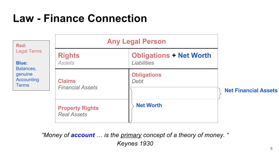
We will not focus on the legal-institutional foundations of monetary economies in this article, but if you are interested in why we translate standard accounting terms to legal terms here, this paper provides some more extensive background. This paper by two japanese colleagues provides some additional useful overall historical background information on the relation between roman law and double entry accounting. John R. Commons’ 1924 ‘Legal Foundations of Capitalism‘ and his 1934 ‘Institutional Economics‘ may be a good starting point for those interested in exploring this important and often neglected topic. Important more extensive recent contributions to legal institutionalism, which we are reconnecting to monetary economics by making explicit the legal character of assets and debt, which hasn’t been done before by legal institutionalists, have been Geoff Hodgson’s ‘Conceptualizing Capitalism’, Katharina Pistor’s ‘The Code of Capital’ and Jean-Philippe Robé’s ‘Property, Power and Politics’. We have also posted a list of online resources on Legal Institutionalism here. Stützel himself in the 1950s built on John R. Commons’ work, but connected it to national accounting and monetary macroeconomics which had developed in response to the great depression of the 1930s, by way of a balance sheet based model of a closed economy – something Commons had not done, and is also lacking in Hodgson’s, Pistor’s or Robé’s work. We follow and develop Commons’ and Stützel’s line of thought here.
So, Financial Liabilities are called ‘debt’ here, and we added the legal terms to clearly distinguish legal rights and obligations (red) from immaterial accounting entities (balancing items, blue), which are mathematically constructed by definition. It is clearly visible here how the balancing item (blue) Net Worth is composed of Real Assets, plus Net Financial Assets (another balancing item).
This trivial accounting relationship now also holds true for flows (changes in stocks over a defined period of time), denoted by a ‘Δ’ (Delta) here:
ΔNW = ΔRA + ΔNFA.
The change in Net Worth ΔNW (also known as profit/loss or, in terms of national income accounting, as saving S) equals the change in Real Assets ΔRA plus the change in Net Financial Assets ΔNFA.
This relationship between flows is equivalent to the relationship used to describe flows of money-denominated wealth in national income accounting for any open economy:
Y- C = S = I + (X – M)
For any period, Income Y minus Consumption C equals Saving S, which equals Investment I, plus Exports (sales of nonfin. assets & services) X, minus Imports (purchases of nonfin. assets & services) M. (X-M) is also known as net exports NX or balance of trade and roughly equal to the current account balance CAB. This implies – as also recognized by MMTers Wray and Tymoigne, for example – that
S = ΔNW
Saving S equals the change in Net Worth ΔNW over a specified accounting period, typically 1 year. In business accounting, yearly saving is determined by the income (profit & loss) statement.
I = ΔRA
Investment I equals the change in Real Assets ΔRA.
Attention: This unfamiliar definition of investment as ‘change in Real Assets is what the term ‘investment’ means in the context of national accounting, only! In business finance, the term ‘investment’ has a different, much more familiar and much broader definition: ‘use of financial means’. It’s important to clearly distiguish these two different definitions! In this article, we will deal with the concept of investment as it’s defined in national accounting, exclusively: Investment I (a flow) equals the change in real assets per period.
(X – M) = ΔNFA
Exports X minus Imports M (net exports/balance of trade (X-M)) equals the change in Net Financial Assets ΔNFA.
In National Accounting, this is calculated in the balance of trade, which is part of the balance of payments statement for a nation. A positive trade balance or trade surplus denotes net exports > 0: a country sold/exported more nonfinancial assets and services (in terms of money-denominated value) than it bought/imported, thus increased his Net Financial Position. An increase of NFP can mean enlarging a net creditor position (as is regularly the case for germany, for example), or diminishing a net debtor position (as was the case for germany when it had to pay war reparations during the 1920s or is the case for Greece today). By the same token, a negative trade balance or trade deficit denotes net exports < 0: a country sold/exported less nonfin. assets and services than it bought/imported, thereby decreased his Net Financial Position. A decrease in NFP can mean diminishing an existing net creditor position (as was the case for the U.S. starting in the 1960s, before its net creditor position vis a vis rest of world turned into a net debtor position in the late 1980s), or enlargening an existing net debtor position (as was the case for the U.S. after 1990 or for Greece in the years following the 2008 financial crisis).
Nota Bene: there are two potential sources of unneccessary misunderstandings here, which I want to clarify up front:
(1) This meaning of the term ‘Investment’ (change in nonfinancial real assets) in the context of national income accounting is DIFFERENT from the meaning of the term ‘Investment’ as used in business practice, where it means ‘use of financial means’. If I buy a government bond on credit from my bank by overdrawing my already overdrawn account, or in exchange for cash, that is an ‘investment’ in the ‘business’ sense of the word, but NOT an investment in the national income accounting sense of the word, as my stock of real (nonfinancial) assets did not change by this transaction. Just like with terms like ‘saving’, ‘money’ or ‘capital’, this ambiguity of the term ‘investment’ often becomes a source of unneccessary (and sometimes also undiscovered) misunderstandings that lead to unneccessary confusion and debate. In this article, the term ‘Investment’ is used only in the sense of ‘change in nonfinancial assets’ ΔRA, which is consistent with standard national income accounting terminology (but not with the more general meaning of the term in business practice).
(2) ΔNFA is not fully equal to (X – M) since besides the balance of trade, ΔNFA also includes net financial transfers. More precisely, ΔNFA is equal to the Balance on Current Account CAB, which besides the Balance of Trade also includes the Balance of Transfers (called Net Revenue from Abroad NRA in national accounting). For the sake of simplicity, I will abstract from this difference in this first run-through of the argument, remembering that we will have to bring this specification back in later to be reasonably precise and to explicitly include the financial sector in the macro model in a realistic way. In most situations, it is quantitatively not so important; it can become important in situations where war reparations have to be served, for example (as after WW I for germany); it can also become important for so-called ‘periphery’ countries as development aid or debt relief received in the form of transfers.
For any closed aggregate economy, there can be no exports or imports by definition, so (ex post), (X-M) will always equal zero. This implies that for any closed agg. economy, S will equal I by definition:
Sagg = Iagg
In terms of business accounting and balance sheet changes, this relationship is equivalent to
ΔNWagg = ΔRAagg
Any closed aggregate economy’s change in net worth ΔNWagg is equal to its change in Real Assets ΔRAagg , as any closed economy’s Net Financial Assets NFA always equal zero by definition – a trivial ex post accounting relationship well known in national accounting, and also in the sectoral balances models of a closed economy as developed in MMT and stock flow consistent modelling.
In terms of stocks, this trivial ex post macro accounting relationship can be visualized like this (we used legal terms here to explicitly reconnect to the sphere of law, as we combine sectoral accounting with an explicit legal institutionalist approach: Financial Assets = Claims, Real Assets = Property Rights, Financial Liabilities = Obligations):
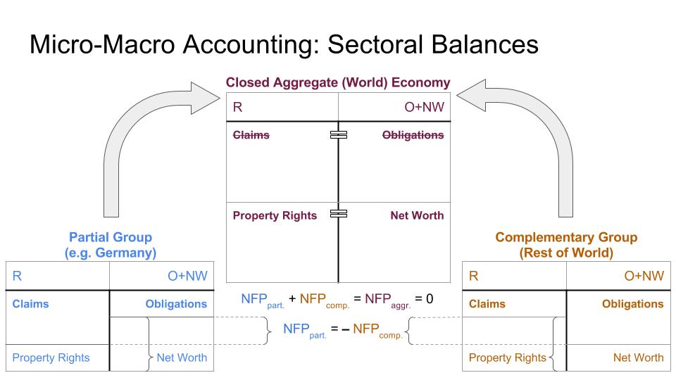
Net Financial Assets NFA (sometimes – as in this slide – more aptly called ‚Net Financial Position‘ NFP since it is a balancing item that can take on both positive and negative values, i.e. become a net asset if > 0 or net debt if < 0) is the crucial link between financial and ‚real‘ spheres. The other crucial balancing item is net worth.
An increase in Net Financial Assets can be accomplished only by achieving a current account surplus, which is roughly equal to a trade surplus, i.e. (X – M) > 0. To be able to achieve that, subjects first need to plan to sell more real assets (in terms of monetary value) and services than they buy.
Sales of real assets or services imply revenues, i.e. increases of net financial assets, purchases of real assets or services imply expenditures or ‚spending‘, i.e. decreases of net financial assets. So to achieve a trade surplus, subjects need to plan to achieve revenues > (greater than) expenditures, or an increase in Net Financial Assets, over the planning period. The terms ‘revenues’ and ‘expenditures’/’spending’ seem to be somewhat ambigous in anglo-american accounting practice, the terminology of which I am not familiar with in much detail. Therefore I need to clarify here that I will use these terms in the following, unequivocal sense:
In german standard business accounting (which Stützel used and which I am familiar with), the terms ‚revenues‘ (‘Einnahmen’) and ‚expenditures‘ (‘Ausgaben’) are unequivocally defined as ‚increases of net financial assets‘ and ‚decreases of net financial assets‘, and unequivocally distinguished from ‘receipts’ (‘Einzahlungen’) and ‘payments’ (‘Auszahlungen’), which increase or decrease the stock of means of payment, and from ‘yields’ (‘Erträge’) and ‘costs’ (‘Aufwendungen’), which in- or decrease net worth:
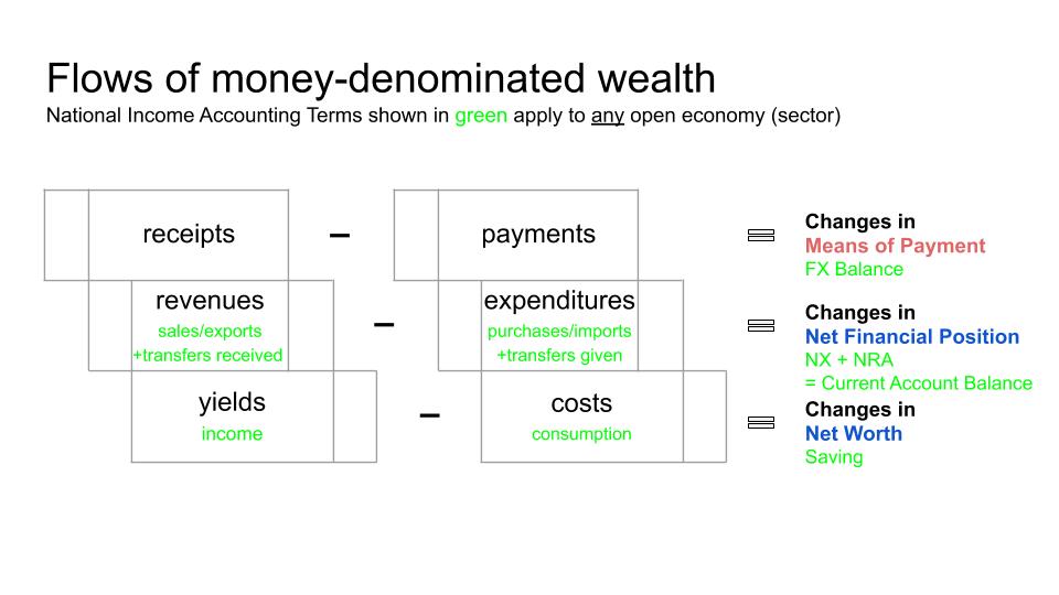
Yields can also be called gross income, costs can also be called consumption. So to say that yields minus costs equal the change in net worth is equivalent to saying that (gross) income minus consumption equals saving: Y – C = S, which is a transformation of Y = C + S.
How is this classification of 3 specific types of ‘moneyflows’ applied to different types of transactions? A systematic look at the major different types of transactions would be necessary to really clearly explain this set of concepts, but for the purposes of this article, I will just focus on a few examples indispensable to clarify Stützel’s arguments re: rentability effect of CB interest rate policy.
If I sell a real asset (i.e. property – some nonfinancial asset or ‘commodity’ which could be some ‘consumption good’ or ‘investment good’), this can happen in three different ways:
(1) If I sell a real asset over the counter at book value and the buyer pays instantly in cash, my real assets decrease and my stock of means of payment (which is part of my financial assets) increases by the same amount. Since the stock of my other financial assets (such as accounts receivable or bonds) and the stock of my financial liabilities did not change, this also increased my net financial position NFP=NFA. My net worth, however, remained unchanged as my increase in net financial assets was offset by a decrease in real assets. So in terms of the above ‘Schmalenbach staircase’ classification of 3 types of flows of money-denominated wealth, this particular transaction would represent a receipt (increase in means of payment) and also a revenue (increase in net financial assets), but not a yield (increase in net worth).
(2) If I sell real assets at book value on account, i.e. on credit, my stock of means of payment will remain unchanged as I do not get paid right away. But my stock of other financial assets will increase as I will book an ‘account receivable’, a claim for means of payment due at some later date against my customer, as a financial asset. And since my stocks of means of payment and financial liabilities did not change, my net financial assets will increase just as they increased when I got paid instantly in cash. My stock of real assets will decrease, which will offset the increase in net financial assets; therefore, my net worth will remain unchanged. This would represent no receipt (stock of means of payment unchanged), a revenue (net financial assets increased) but no yield (net worth unchanged). When my customer finally pays his bill 30 days later, I lose my claim (‘account receivable’) against him, but gain means of payment of the same amount. This payment transaction is a purely financial transaction that does not change the quantitative amount of my net financial assets, but only its qualitative structure in terms of risk, maturity and liquidity composition. The actual payment of debt therefore represents a receipt, but not a revenue and not a yield.
I presupposed sales at book value and zero interest for the sale on credit for the sake of simplicity and clarity here. It would be no problem to give additional examples where commodities are sold above book value and on credit for which interest is being charged. You, the reader, might want to do this and determine the amounts of the 3 types of flows these transaction would create, in order to test your understanding of Schmalenbach’s distinction of 3 types of moneyflows depicted above. It is a core part of Stützel’s clarification of accounting terms within Keynesian ‘monetary production’ type circuit models of a closed economy and the interaction of real and financial spheres. Now let’s move on to example 3:
(3) If I sell a nonfinancial asset or service at book value to one of my creditors, I receive a claim against him: we can then agree to settle that claim by offsetting (netting) it with a liability I have towards him. In that case, my net financial assets increased because my stock of fin. liabilities decreased. Again, even though I paid (settled) with my customer, my stock of means of payment did not change. The transaction represented no receipt, but a revenue, and no yield. In this transaction, no actual means of payment were involved but a payment (settling) happened nevertheless: actual payment was substituted by offsetting of claims.
[For a systematic look at the different ways a payment obligation can be discharged with or without any ‘money’ in the sense of ‘means of payment’, we strongly recommend Borja Clavero’s paper ‘Money and Hierarchy: 4 Ways to Discharge a Payment Obligation’. Together with Mehrling’s paper on the hierarchy of money, it has essential clarifications for precisely distinguishing ‘money’ in the sense of ‘credit’ from ‘money’ in the sense of ‘means of payment’ and a systematic understanding of all the different operations by which payment obligations can be discharged.]
Note that only one of these transactions changed my stock of means of payment. But they all changed my net financial assets, therefore represented revenues. Had I sold some service, the only difference would have been that this would also have increased my net worth since my increase in net financial asset would not have been offset by a corresponding decrease in real assets. Therefore, we can say: real assets or services are always exchanged for ‘money’ in the sense of net financial assets. But they are not always exchanged for ‘money’ in the sense of means of payment! The latter is true even though payment obligations are claims for means of payment and must eventually be ‘paid’ – as we showed above, offsetting/netting offers one of the ways this can happen without any means of payment being involved. And one core function of banks and the banking system, besides their standard function of let size, risk and maturity transformation which is sorely neglected in MMT, is simply that they also act as clearinghouses: as institutions that facilitate multilateral netting between other economic subjects.
We can conclude that in a realistic macro circular flow model of a closed economy, the flow of ‘real assets and services’ in one direction is mirrored by a corresponding flow of ‘money’ in the sense of net financial assets (not in the sense of means of payment, which needs to be looked at separately) in the opposite direction. This flow of net financial assets is often followed by a flow of means of payment at some later date, but not always, as payment can happen by bilateral offsetting as well. And depending on how the payment is carried out, it can lead to an increase, a decrease or no change of M1. Therefore, changes in net financial assets and changes in the stock of means of payment need to be looked at separately. Stützel called this the ‘bipartite division of the object of the theory of money‘, as the two different flows are often conflated in the ambigous term ‘money’, creating unneccessary ambiguity and confusion.
We need to conclude at this point that since real assets and services are not always exchanged for ‘money’ in the sense of ‘means of payment’, but are always exchanged for ‘money’ in the sense of net financial assets, net financial assets (and not means of payment) is the critical missing link between the financial and the real sphere. The term ‘money’ is much too ambigous for developing any precise understanding of the financial system and its interaction with the nonfinancial ‘real’ sphere of nonfinancial assets and services.
The term ‘money’ therefore should never be used without further specification (‘money in the sense of … means of payment, commodity means of payment, credit means of payment, credit, net financial assets, etc.). Better, yet, is to not use the term ‘money’ at all, but simply substitute the precise distinction one actually means in order to avoid unneccessary misunderstandings and confusions created when one speaker uses an ambigous term, and different listeners interpret it differently, assuming they understood what the speaker meant. Economic history is full of such ambiguities – in this article, we demonstrate some steps to clarity Stützel took for the terms ‘money’, ‘saving’, ‘price’, ‘demand & supply of goods & services’ by applying precise distinctions and definitions, to clarify some core issues in keynesian and post keynesian debates.
But let’s now return to an aggregate perspective.
Ex post, aggregate sales/exports (revenues) and aggregate purchases/imports (expenditures) will of course be equal by accounting identity: my $ 1000 sale equals rest of world’s $ 1000 purchase, and that’s the case for all other sales as well. Generally, the following ex post accounting identities are true by definition:
Xsectorex post = Mrowex post
Ex post, any sector’s actually completed sales/exports equal rest of world’s actually completed purchases/imports.
Msectorex post = Xrowex post
Any sector’s actually completed purchases/imports equal rest of world’s actually completed sales/exports.
Xsectorex post + Xrowex post = Xaggex post
Any sector’s actually completed sales/exports plus rest of world’s actually completed sales/exports equal aggregate sales/exports.
Msectorex post + Mrowex post = Maggex post
Any sector’s actually completed purchases/imports plus rest of world’s actually completed purchases/imports equal aggregate purchases/imports.
Xaggex post = Maggex post
Ex post, aggregate sales/exports are equal to aggregate purchases/imports.
So far, so good. Up to this point, probably most MMTers would agree and go along with this. But now I will introduce a crucial distinction Stützel made that I have not seen as clearly and systematically in any MMT texts, and that is the distinction between ex ante planned flows and ex post actually achieved flows. An obvious example would be a company that ex ante, in the beginning of 2022, plans a total of $ 10.000.000 worth of sales for next year (2022), therefore supplies (produces and offers) $ 10.000.000. worth of commodities for 2022. The same company might plan to purchase commodities and services worth $ 8.000.000 for that year, in other words, to demand $ 8.000.000 of commodities and services. Supply and Demand are ex ante categories! But end of December 2022, when it closes its accounts, it may notice it ex post only actually achieved sales worth $ 9.000.000 – $ 1.000.000 less than it had planned (with the rest of unsold commodities filling its inventory). Total purchases may ex post (at the end of the year) also deviate from what was planned ex ante (in the beginning of the same year).
These ex ante categories: planned purchases = planned expenditures (planned decreases of net financial assets) = demand for goods and services and planned sales = planned revenues (planned increases of net financial assets) = supply of goods and services also can be aggregated within a closed economy model to obtain ‘aggregate demand’ (aggregate planned decreases in NFA) and ‘aggregate supply’ (agg. planned increases in NFA).
We found above that ex post, aggregate sales/exports are always equal to aggregate purchases/imports by accounting identity. On the ex ante level of future plans, however, there is no such accounting identity! Rather, aggregate planned exports/sales of nonfin. assets & services (= planned revenues) also known as ‘aggregate supply‘ – and aggregate planned imports/purchases of nonfin. assets & services (planned expenditures) also known as ‘aggregate demand‘ can deviate from each other (and thus, be incongruent with one another) for the simple reason that in a market economy, independent ‚free‘ legal subjects plan independently from one another: they do not coordinate their plans ex ante, but plan independently on the basis of vaguely anticipating, but not fully knowing everyone else‘s plan. So if I plan to sell $ 10 000 worth of real assets and services and ‘supply’ those, there is no guarantee that rest of world plans to buy $ 10 000 worth of real assets &services from me. It may very well plan to buy $ 11 000 or $ 9 000 worth of real assets and services from me, therefore ‘demand’ more or less than I ‘supply’. If rest of world plans to buy less than I plan to sell, I may try to persuade them into planning to buy more (by advertising and other means). But I certainly have no way into ‘making’ them plan to buy as much as I plan to sell ‘by accounting identity’. Michael Pettis, who actually (mistakenly) believes that ‘supply and demand are equal by accounting identity‘ seems to have trouble understanding this very pedestrian everyday fact of any ‘free market’ economy based on decentralized planning and contract! This misunderstanding is clearly a case of misinterpreting accounting identities by failing to make the distinction between ex post flows (where the accounting identities always apply as long we are in a closed economy using 1 single currency or fixed exchange rates) and ex ante planned flows (this is the category into which the concepts of ‘demand’ and ‘supply’ belong), where there are no such accounting identities whatsoever.
Plan coordination happens ex post on the market when subjects try to realize their plans; and incongruent plans will lead to market tensions, price negotiations, and may lead some subjects to decide to sell or buy at a price different from the price they had planned to sell or buy at (decisions often described by the misleading metaphor ‘price mechanism’). As anyone knows, this kind of decentralized ex ante planning, plus plan coordination via the free market and the ‘price mechanism’ is the very basic principle of any private (property&contract) law based free market economy.
Aggregate ex ante planned sales of real assets (planned exports) is synonymous with aggregate planned revenues and aggregate ‚supply‘ of real assets; aggregate ex ante planned purchases of real assets (planned imports) is synonymous with aggregate planned expenditures (‚spending‘) and aggregate ‚demand‘ for real assets. That supply and demand are ex ante categories referring to plans is even clear on the level of pure semantics: if I supply commodities, I have them in stock (‘in supply’) and plan to sell them and therefore offer them – but I haven’t sold them yet. If I ‘demand’ commodities, I plan to buy them – but I haven’t bought them yet. If I had already bought them, I would already own them and therefore would not need to ‘demand’ them in any way from someone else. Therefore, even on a purely semantic level, demand and supply are clearly EX ANTE categories.
To summarize: for a period t1 … t1+x, we can say:
(A) EX ANTE (t1):
Xaggex ante/planned > or < or = Maggex ante/planned
Aggregate supply Xaggex ante/planned can (and usually will) be greater or smaller than aggregate demand Maggex ante/planned; they will be equal only in an unlikely special case. This (unlikely) special case where both equal each other is usually called ‘equilibrium’.
(B) PRODUCTION, SALES/PURCHASES (t1 … t1+x) – Subjects act to turn their (t1) plans into reality. When trying to sell their products, they encounter the plans of ‘rest of world’, which may or may not match their own plans.
(C) EX POST (t1+x):
Xaggex post = Maggex post
Ex post, actually completed aggregate sales/exports will always equal actually completed aggregate purchases/imports, by definition: this is not some kind of ‘equilibrium’ that could be deviated from, but an accounting identity simply true by definition. If in t1, Xaggex ante/planned had been > or < Maggex ante/planned , then in t1+x some of those plans will have failed: they could not be realized.
As far as my MMT understanding goes, in MMT, the concepts of supply and demand for real assets & services are not yet coherently related back to the sectoral accounting framework in this conceptually and semantically coherent way. Sometimes one gets the impression that MMTers see ‚spending‘ as such as synomous with ‚demand‘ for real assets, not distinguishing ex post actual spending from ex ante planned spending explicitly and systematically enough. The former can be traced back to balance sheet entries as they relate to transactions that have already happened. The latter cannot be traced to balance sheet entries, as it relates to transactions that have not have happened yet.
This distinction is crucial, however. Aggregate demand cannot be equal to ex post aggregate spending: in that case, aggregate supply would have to be equal to aggregate revenues, and we know that aggregate ex post expenditures are always equal to aggregate ex post revenues by accounting identity. So if agg. ex post expenditures would be equal, aggr. aggr. demand could never deviate from aggr. supply – they would always be equal by definition, which would imply that things like the great depression could have never happened.
So if the CB raises the interest rate above the average rate of expected yields on nonfinancial assets, this will most probably induce firms to plan trade surpluses for the following period: a plan to restructure their portfolio to maximize profit, as holding wealth in the form of net financial assets promises profits higher than holding it in the form of nonfinancial assets. If agg. planned trade surpluses > planned aggregate trade deficits, this amounts to aggregate supply for real assets being > aggregate demand.
The same plan constellation of agg. planned revenues (supply) being greater than agg. planned expenditures (demand) can also be expressed as aggregate planned change in net financial position being > 0, or as the familiar Keynesian
S desired > I desired
Again, this simply results from S = ΔNet Worth (NW) and I=ΔReal Assets (RA):
NW = RA + FA – FL
Net Worth equals Real Assets plus Financial Assets minus Financial Liabilities, and
FA – FL = NFA
Financial Assets minus Financial Liabilities equals Net Financial Assets so that
NW = RA + NFA
Net Worth equals Real Assets plus Net Financial Assets. This also holds true for flows / changes in stocks:
ΔNW = ΔRA + ΔNFA
The change in Net Worth (profit/loss; yields/period minus costs/period) equals the change in Real Assets plus the change in Net Financial Assets.
Therefore, S (ΔNW) can deviate from I (ΔRA) only if ΔNFA deviates from zero.
For any closed aggregate economy as a whole, therefore, ex post, S will always equal I by accounting identity, as NFA of a closed aggregate economy must always equal zero by definition and can never deviate from zero: this is a trivial standard insight in national accounting, as well as in MMT or stock flow consistent models. Therefore,
Saggex post = I aggex post
is nothing but a trivial ex post accounting identity.
Ex ante, however (in terms of ‘desired’ or ‘planned’ S and I), Sagg and Iagg can and typically will deviate from one another, as in private law based market economies, planning is by definition decentralized and autonomous for every legal subject, so that legal subjects plan independently from one another, only anticipating everyone else’s plans without fully knowing them and without coordinating their individual plans ex ante. Plans get coordinated only in the phase of their realization by way of supply/demand incongruencies and the so-called ‘price mechanism’ – a (sometimes misleading) metaphor for price negotiations and decisions. Negotiations and decisions are intentional human actions, not some ‘mechanism’ and depend on power relations generally, not just in monopoly situations. We will look at two particular types of such power relations: buyer’s market and seller’s market tensions, in more detail below.
For any open economy (individual firm or sector), S and I can deviate from each other ex post. Sex post will deviate from Iex post by ex post net exports (X-M)ex post, as S = I + (X-M). Exports X are sales of real assets to rest of world, imports M are purchases of real assets from rest of world. The ex post accounting identities are Xsector = Mrest of world (any sector’s exports/sakes equal rest of world’s imports/purchases) and vice versa, so that ex post,
(X-M)sectorex post = -(X-M)rest of worldex post
(X-M)sectorex post + (X-M)rest of worldex post = 0
or
(S-I)sectorex post = -(S-I)rest of world ex post
(S-I)sectorex post + (S-I)rest of worldex post = 0
Which in turn are just 2 more ways to express the standard ex post accounting identity regarding net financial assets (NFA):
ΔNFAsectorex post = -ΔNFArest of worldex post
Any sector’s change in net financial assets equals rest of world’s negative change in net financial assets by accounting identity. Therefore,
ΔNFAsectorex post + ΔNFArest of worldex post = 0
Any sector’s change in net financial assets plus rest of world’s change in net financial assets add up to zero, as the closed aggregate economy’s net financial assets equal zero at all times, by accounting identity (i.e. by definition).
Of course, we can subdivide into any other number of sectors: we could disaggregate the closed aggregate economy into the sectors used in standard national accounting (government, private nonfin. businesses, priv. fin. businesses, priv. households, foreign), or right down do each individual legal subject. The ex post accounting identities would remain the same. I’m sticking with only 2 sectors for simplicity, here. The basis of this simple use of standard ex post accounting terms is well established in MMT, albeit not always as explicitly integrated with national income accounting categories as described above, and not always clearly distinguishing ex post from ex ante variables (which is crucial, see below). Compare for example the section on ‘macroeconomic accounting’ in Tymoigne/Wray’s 2013 ‘The Rise of Money Manager Capitalism’, p. 20-21.
But ex ante, in the planning stage, the above aggregate balances will equal zero only in a very unlikely special case. Usually, they will deviate from zero.
Xplanned are planned sales to /revenues from, Mplanned are planned purchases from/expenditures to rest of world.
So if on the aggregate level,
Xaggpl > Maggpl
aggregate planned sales / revenues are > agg. planned purchases / expenditures, then
Agg. Supply > Agg. Demand
This implies that
(X-M)aggpl > 0
the closed economy (world as a whole) plans a a trade surplus (which it by definition cannot achieve as for a closed economy, there is no external trading partner by definition, so its balance of trade can only be zero at all times), and
Saggpl > Iaggpl
the world as a whole plans to save more than to invest (the classic Keynesian version of the paradox of thrift), which is also impossible to achieve since ex post, S will be equal to I by accounting identity, so that some plans will have failed ex post; and
ΔNFAaggpl > 0
the world (closed aggr. economy) as a whole plans to increase its net financial assets, which is also impossible to achieve since ex post, the aggregate economy’s change in NFA will be zero by definition.
This last insight is well known and well established in MMT; but I haven’t seen it expressed as the synonymous Spl > Ipl or as Xpl > Mpl anywhere in MMT (as of Dec 2020; in case any MMTers described this anywhere, please let me know by commenting below).
So, let’s summarize: the constellation
Aggregate Supply > Aggregate Demand
(for ‘real’ assets & services)
can also be described as
Xaggpl/ex ante > Maggpl/ex ante
Aggregate planned exports/sales (of real assets and services) are greater than aggregate planned imports/purchases;
(X-M)aggpl/ex ante > 0
Aggregate planned net exports/balances of trade are greater than zero;
ΔNFAaggpl/ex ante > 0
Aggregate planned changes in net financial assets are greater than zero, or finally as
Saggpl/ex ante > Iaggpl/ex ante
All of these expressions are synonymous: different ways of describing the same constellation of incongruent aggregate plans re: buying&selling nonfinancial assets & services (i.e., aggregate demand & supply).
What can we say about what the outcomes of such incongruent, not fully achievable plans will be?
If aggregate plans to increase net financial assets are > 0, this will mean ex post some plans must fail as ex post, the change in net financial assets of any closed economy always equals zero, by definition (by accounting identity). If aggregate planned sales are > aggregate planned purchases, either some planned sales will not have been realized ex post so that ex post (t2) achived sales < sales that were planned in (t1) for the period (t1 … t2). Or aggregate planned purchases will ex post (t2) be greater than was planned ex ante (t1) for the period (t1 … t2).
That crucial (and fairly trivial) relevance of the ex post macro accounting identities of the sectoral accounting framework is – as far as I‘m aware, and correct me if I m wrong – not yet explicitly and precisely described or used this way in MMT discourse. It was, however, a standard insight in any german national accounting textbook of the 1960s, such as Alfred Stobbe‘s ‚Volkswirtschaftliches Rechnungswesen‘ (1966, p. 130ff)! But as a reaction to 1970s stagflation, economics turned away from the accounting based macro models that had been developed following the great depression of the 1930s (with notable contributions by Wassily Leontief, James Tobin, Lawrence Klein and others), throwing the baby out with the bath water instead of improving them so they could accomodate stagflation. This is a crucial failure of the keynesian & post keynesian tradition to this day in our opinion, and one that Stützel remedied in a quite simple and trivial, but as yet largely unrecognized way (see below).
To explore some consequences, let‘s first use the standard implicit Keynesian presupposition of ubiquitous buyers’ market tensions (where buyers – the ‚demand side‘ – have power over sellers – the ‚supply side‘), as that will be an uncontroversial assumption for people considering themselves Keynesians: the ‘demand-led’ economy, where changes in aggregate demand determine changes in output and employment. New for Keynesians will only be Stützel’s insight that this is an unexplained general assumption generalized mostly from the great depression period where this was indeed the case in an extreme way, and, although in fact a (very frequent) special case, not a ‚natural fact‘ and ‚general‘ case, and therefore requires an explanation based on a careful collection of historical counterexamples (which I will only cover shortly in this short sketch).
In that particular situation, demand (plans to buy nonfin. assets & services) will win over supply (plans to sell nonfin. assets & services): planned purchases (planned spending) determine ex post realized sales (planned revenues), so that the result will be that some planned sales will ex post not have happened as was planned. Ex post, some revenues that had been planned ex ante will not have been been achieved as planned.
Total planned sales are equal to total quantity of real assets to be sold, multiplied by price. So either, not all real assets that were planned to be sold ex post could be sold: some firms, at the end of the period, still have some products left in their stock which they originally had planned to sell. Or, the other possibility: all real assets were actually sold as planned – but some of them could only be sold at a price lower than the price that was planned ex ante.
In that latter case, the price level will most likely have dropped (‘deflation’, as during the 1930s great depression) as a result of the raised interest rate, not risen.
Now if in the next period, the CB will keep interest rates – expected yields/period on fin. assets – above the average expected net yields/period on real assets, and firms continue to maximize their profit, plans will remain at the same constellation. But those who failed to achieve their plans will probably try to achieve their plans next period by reducing their expenditures (i.e. by trying to be more economical with their raw materials and labour by improving workflows and work organization, and/or negotiate lower prices for the labour, raw materials and pre-products they need for production during the next period, reduce their purchases of investment goods, etc.). They will concentrate on the expenditures (RA purchases/demand) side as the expenditures/demand side wins on buyers’ markets.
This will (ex post) lead to a drop in aggregate expenditures (which equal aggregate revenues – not aggregate income !! – by accounting identity), with again the same result of some failed plans as above etc. If buyer’s market tensions prevail, ex post aggregate expenditure/revenue will be a function of aggregate planned expenditure (aggregate demand). This self-accelerating process can lead to a deflationary spiral of declining total expenditures that should be familiar to any Keynesian from the 1930s. It was the experience of the 1929ff. great depression, for which the ‘classical theory’ (for Keynes, classical economics including Marx, and the Walrasian ‘neoclassical’ tradition of his time) had no explanation, that led Keynes to write his 1936 ‘General Theory of Employment, Interest and Money’ in the first place.
From Stützel’s point of view, it is this strategy that leads to a change in total expenditures/period, not some ‘mechanics of ‘money’ creation’ or a mistakenly supposed accounting identity of aggregate supply and aggregate demand.
If in that situation, governments plan additional expenditures / purchases of nonfin. assets (of bombs or whatever – as we know, in the later 1930s, in increasingly became bombs, tanks etc.), it can change aggregate plans so they will either be congruent (‚equilibrium‘) or even aggregate demand > aggr. supply. In that case, the above process reverses, and as long as firms still expect & experience buyers’ market tensions, total expenditure/production will rise, not necessarily the price level.
But the plan constellation could also be changed if central banks lower interest rates significantly below the average expected net yields on real assets. But if average expected net yields on real assets are very low already, there is little room to manouver with interest rate policy, and fiscal demand stimulus policy – planning additional gov‘t expenditures – must help out (which is what Central Bankers had been calling for since 2019, at least). In that sense, what has been missing over the past decades of low interest rate policy was adequate coordination of monetary and fiscal policy.
Now, imho this is all pretty much compatible with standard Keynesian theory. For Keynes, ‘marginal efficiency of capital’ meant that money interest rate is equal to the net rate of returns (net yields) expected from the purchase of additional real investment assets. A firm will employ additional real investment assets only if it expects its net yields to be greater than the interest owed for financing them. Therefore, lowering the money interest rate can c.p. lead to more investment plans actually being carried out because more of them promise net yields > money interest rate.
It is also congruent with how Central Banks actually have learned to conduct monetary policy via changing short term interest rates in practice, and are doing monetary policy today– and I don‘t see how to square that with Mosler‘s imho confused claim + added ad hoc ‚theorizing‘ that
‚Monetary policy has it backwards – raising interest rates is actually expansionary, lowering them is actually contractionary‘ (verbatim quote from video linked at the beginning of this article).
Based on the view sketched above (and further below), it seems to me that quite the contrary could be the case: it seems to be Mr. Mosler who ‚has it backwards‘ even by Keynesian standards (let alone by standards of actual central banking practice).
I find this a little surprising for someone claiming to be an expert on ‘money’ and monetary policy, and someone claiming his views to be compatible with Keynes’ thinking.
To see that more clearly, let’s take Stützel’s view one step further: once buyers’ market tensions are dismanteled and sellers’ market tensions develop, which will inevitably happen if average expected net yields on real assets consistently remains above expected average yields on net financial assets and therefore, nonfin. firms consistently plan to achieve their profits by trade deficits (by decreasing net financial assets): then, power will move over to the sellers’ side (sellers’ markets) and the choice to raise prices will be preferred by sellers, which eventually will lead to stagflation.
Buyers’ markets also put pressure on producers regarding product quality, customer service, efficient organization of work and efficient use of resources. Sellers have to try to persuade and ‚bribe‘ buyers into buying their stuff (we all know the kinds of presents sellers sometimes offer in that regard). Sellers’ markets remove that pressure from sellers put it on buyers – customers. They now have to run after sellers, bribe them to get the products they want, and stand in line in the shops – a well known phenomenon seen in an extreme form in 1970s & 80s real socialism, analyzed by Janosz Kornai in his 1980 ‘Economics of Shortage’ (summary presentation here), and even re-emergent today in some countries, notably in Venezuela in an extreme form). Product quality declines, delivery times get longer. In the 70s, mild forms of that could be witnessed during the stagflation era in capitalist economies as well (I very well remember the relatively low level of customer service at the time, as compared to today’s level).
As Stützel noticed in 1953, this is not clearly conceptualized by Keynesians yet because to them, buyers’ market tensions are something ‚natural‘ and ‚ubiquitous‘, whereas sellers’ market tensions exist as little for them as for their Walrasian foes; see his ‘Paradoxa der Geld- und Konkurrenzwirtschaft’ ´(written in 1953, published only in 1979), p. 182-199). Unfortunately, the latest article on Stützel’s theory of business cycles by Johannes Schmidt in the Journal for the History of Economic Thought knowingly simply denies Stützels sellers’ market cases, thereby willfully misrepresenting Stützel’s work and distorting economic history, ironically by omitting Stützel’s innovation beyond Keynes and incompletely portraying him as a ‘pure Keynesian’. By re-generalizing to the old keynesian ‘buyer’s markets as the general case’, Schmidt tries to eliminate Stützels explanation of additional cases, while still accomodating the Keynesian cases as special cases. Stützel followed the same integrative methodological strategy here (and in all of his work) that Keynes used in the General Theory (see GT, preface and Chap. 1): accommodate the cases described by previous theories as special cases by making explicit their implicit assumptions, then explain additional cases within a corrected general conceptual framework that allows for this. Schmidt eliminates integrative the theoretical progress Stützel made here. We know from personal discussions with Schmidt that he knows Stützel’s framework of 2 buyers’ market and 2 sellers’s market cases very well, but does not share it. Nevertheless, in an article for a Journal for the HISTORY of economic thought, he would have had to represent Stützel’s model completely and accurately, no matter if he personally shared it or not. This is about honestly and accurately writing the history of economic theory! Schmidt did not do so. By this, he compromised his own scientific integrity for the usual corruption that is practiced within the keynesian camp no less than in the orthodox camp. One of the purposes of this article is to correct Schmidt’s omission.
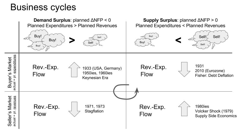
So, in the following 4-way matrix, the two Keynesian ‚buyers’ market tension‘ cases can be found in the top row, the two ‚anti-keynesian‘ ‚sellers’ market tension‘ ones in the bottom row. The historical illustrations were not given by Stützel. I have added them in an attempt to integrate & clarify Stephan Schulmeister‘s Keynesian model of ‘long business cycles’ alternating between ‘real capitalist’ (left column) and ‘finance capitalist’ (right column) phases (summarized here) by viewing it through the lens of Stützel’s scheme.
As Stützel put it,
‘Pure General Equilibrium Theory cannot give a solution for any of these 4 cases of plan divergences. Keynesian Theory only knows the two buyers’ market cases’. (W. Stützel 1953: Paradoxa der Geld- und Konkurrenzwirtschaft, Aalen 1979, p. 188)
And:
‘If economic subjects in a closed economy are planning to decrease aggregate net financial assets, this does not self-evidently – and as claimed by most theories of business cycles – lead to an increase in ex post total expenditures/revenues. This only happens under the special conditions of prevailing buyers’ market tensions. If sellers’ market tensions prevail in the closed economy, the same plan divergence (planned expenditures/sales/purchases or agg. demand > planned revenues/purchases or aggr. supply which implies planned increases of aggregate net financial assets) leads to the opposite result: ex post, the flow of total expenditures/revenues will decrease. ‘ (R.D. Grass/W. Stützel 1988: Volkswirtschaftslehre – eine Einführung, München: Vahlen, p. 341).
To my knowledge, Stützel provided a few historical examples for sellers’ markets (the german post WWII situation before the 1948 currency reform, with a hyperinflating Reichsmark and administered prices was well within his biographical experience), but did not explicitly specify conditions which would lead to sellers’ markets. But imagine an economy where expected yields on financial assets are kept below expected yields on real assets by constant application of fiscal stimulus and low interest monetary policy. This would keep aggregate planned investment > planned saving, and after providing a stimulus as long as buyers’ market tensions exist, dismantle existing buyers’ market tensions, and start to develop sellers’ market tensions. If not stopped by countercyclical monetary and fiscal policy, this may develop into an extreme situation like in Venezuela under Maduro, with a ‘shortage economy’ a la late real socialism, and hyperinflation.
From my point of view, this enables a coherent take on why the keynesian ‘real-capitalist’ constellation (upper left quadrant), while initially being beneficial, will undermine itself and become dysfunctional in the longer run (bottom left quadrant) as it did in the 70s, just as much as its counterpart, the ‘finance-capitalist’ constellation, will be initially useful (bottom right quadrant), but then eventually undermine itself and become dysfunctional as well (top right quadrant). Those may be seen just as normal dialectical life cycles, like inhaling-exhaling, waking – sleeping, tension-release, training-resting, etc. – cycles you want to manage in a way so they don’t get overexaggerated in amplitude. You WANT normal mood swings, anything else would be boredom. But you don’t want to become manic-depressive. You WANT to alternate training and resting, but you don’t want to get into a cycle of overtraining til injury, then resting and couchpotatoing until you get hopelessly overweight, then restart the cycle. That’s why countercyclical monetary and fiscal policy makes sense imo.
One actually fairly trivial, but nevertheless clarifying takeaway insight from this is, in my view: Keynesian policy can only work after buyers’ market tensions were created, first; and this can happen only by aggregate supply (planned revenues) being > aggregate demand (planned expenditures), which will be a result of expected yields on financial assets > expected net yields on real assets. Constant application of demand stimulus policy, of trying to keep aggregate demand > aggregate supply by way of fiscal or monetary policy, will remove the preconditions for that very policy to lead to the desired results, and eventually produce the opposite result: instead of growing output and employment, declining output and employment stagflation, with rising prices.
Which leads to the quite trivial insight that what’s needed is anti-cyclical monetary and fiscal policy that aims at regulating market tensions, i.e. the level of pressure/challenge or ‘discipline’ sellers are faced with in the economy. Which monetary policy already routinely practices by way of a symmetric inflation target, for example, with fiscal policy currently (as of 2020) experiencing a return to the (pre-Stützel) Keynesian policies of the 1930s-60s, based on pragmatic recommendations by today’s central bankers, today’s IMF or even Larry Summer and Olivier Blanchard.
Also note that buyers’ market tensions are good for buyers, bad for sellers. But firms and individuals always are a seller as well as a buyer, if only a seller of labour. Market tensions are particularly crucial for labour markets: buyers’ market tensions (underemployment, as in 1930) weaken union power and strenghten employer’s power, sellers’ market tensions (full employment or labour scarcity, as at the end of the 1960s) strenghten labour unions’ bargaining power and political influence.
I‘d say that this provides a more balanced, integrative perspective beyond the typical quarrel between Keynesians and Anti-Keynesians. That was Stützel‘s explicit goal – much like Keynes, he didn‘t go for a ‚heterodox alternative‘ but for a ‚General Theory‘, and he pursued that goal methodically and had methodical tools he used for that (today‘s ‚heterodox‘ and ‚orthodox‘ economists seem to lack those tools and stuck in their unproductive fighting an in-grouping).
The (trivial) ex post accounting foundations of this view are the same as those of MMT, but Stützel makes some additional explicit precise distinctions MMT does not (yet?) make: distinctions between
- ‘spot’ prices relating to a point in time, like sales prices, and ‘holding’ prices relating to a period of time, like expected net yields on financial and real assets
- ex post accounting identities and ex ante planning deviations from those identities, resulting in the development of
- buyers’ market tensions and seller’s market tensions
This not only coherently relates the concepts of aggregate demand & supply back to the balance sheet based sectoral accounting framework, which MMT does not yet do as far as I can tell. It also integrates Keynes’ thoughts on the role of the interest rate in relation to expected net yields on real assets (investment goods), while Mosler’s claim seems to contradict Keynes here. The model is only very abstract and would need to be specified by including the private household sector, assumptions about their typical portfolio choices, a closer look at the components of net yields on nonfin. investment goods (including wages, for ex.) etc., but the basic patterns of this view have hopefully become clear in this short description.
Stützel also uses a model building strategy of specifying areas of applicability of generalizations, which can demonstrate seemingly incompatible generalizations are actually compatible if their area of applicability is specified; in addition, Stützel looks for implicitly assumed generalizations (like the Keynesian implicit generalization of ubiquitous permanent buyers’ market tensions, thus ‘demand dominance’) to then demonstrate to which special cases they apply and to which special cases they do not apply.
So for example, while Keynesians criticize Say‘s Theorem (‚any supply will always find demand‘) and simply replace it with a reverse Say‘s theorem (‚any demand will always find supply‘), generalizing from the historically specific experience of the great depression mainly, this model specifies the situations where each of the theorems applies (Keynes: buyers’ markets, Say: sellers’ markets).
The debate over which of them is ‘true’ and which is ‘false’ becomes unneccessary and can be recognized as blocking integrative progress/learning, because it avoids asking the question: ‘which statement applies to which specific set of situations‘. Within the framework shortly sketched above, both are true AND false – true for those situations where they apply, false for those situations where they do not apply. By specifying their respective areas of applicability, we see more clearly; by fighting for binary true/false beliefs, we block and avoid seeing more clearly.
I‘ll close here, not very confident in that anyone of the few who may actually have read this up to this point will make any sense of this. I‘ve tried this many times and the reactions were mostly, people at best used what fit their preconceived beliefs and ignored the rest. Only in one case, someone asked, ‘I’d really like to know how these sellers’ market cases work’ but then didn’t pursue the question further, but instead of inquiring how these can be produced went back to presupposing they ‘usually don’t exist’ – where Venezuela would have been a current example with an inflation rate way above the interest rate, where people of course plan to purchase more nonfinancial assets than they plan to sell, and everyone plans to reduce their net fin. assets, producing sellers’ markets (empty shelves in supermarkets etc.).
I’m not a professional economist, so I don’t have the time and resources to engage in constant debate with professionals, or translate Stützel’s entire work. I would have no chance whatsoever anyway against their skilled rhetorical manouvers. However, I do take the freedom as a citizen to express doubt to economists’ claims if I see good reasons for that, whether they come from orthodox or heterodox economist. I also take the freedom to read economists whom I feel made significant contributions to some progress in understanding.
It seems to me that Stützel‘s work was most often used selectively by Keynesians and Anti-Keynesians, who just picked out what fit their theories anyway but ignored the rest, and chose to perpetuate that quarrel between Keynesians and Antikeynesians, and between Orthodoxy and Heterodoxy Stützel wanted to solve rationally by integrative model building a la Keynes’ ‘General Theory’. He was very frustrated with how economics developed during the 70s and 80s.
I the end, I think, power claims will probably always trump attempts at integrative understanding overall, at best, only few people will want to sidestep those power games the way Stützel did, even though we should expect that of any academic economist. I don’t see any of Keynes’ or Stützel’s caliber on the horizon right now who could foster integrative progress in economics, so the divide between orthodoxy and heterodoxy both Keynes and Stützel wanted to bridge will probably continue to exist, and citizens and politicians will continue to tend to distrust most economists and their diverse promises, while themselves relying on uninformed models often containing fallacies of composition, but incoherently muddle through somehow in practice, changing ideologies ad hoc as needed.
Keynes famously wrote in Chap. 24 of his General Theory:
“… the ideas of economists and political philosophers, both when they are right and when they are wrong, are more powerful than is commonly understood. Indeed the world is ruled by little else. Practical men, who believe themselves to be quite exempt from any intellectual influences, are usually the slaves of some defunct economist. Madmen in authority, who hear voices in the air, are distilling their frenzy from some academic scribbler of a few years back. I am sure that the power of vested interests is vastly exaggerated compared with the gradual encroachment of ideas. Not, indeed, immediately, but after a certain interval; for in the field of economic and political philosophy there are not many who are influenced by new theories after they are twenty-five or thirty years of age, so that the ideas which civil servants and politicians and even agitators apply to current events are not likely to be the newest. But, soon or late, it is ideas, not vested interests, which are dangerous for good or evil.” (full text here)
I used to believe that too. But these days, after observing both political discourse and post 2008 academic discourse, I tend to conclude that Keynes may have overestimated economist’s influence. Much more than their ideas, power relations influence what happens, and pragmatic elite reactions and changes of ad hoc opinions, legitimated by pretty much randomly chosen ideology, in reaction to crises. Sure, Keynes’ belief may have boosted his self-image as well as that of his colleagues (‘it’s us who make history with our ideas’). I tend to think these days that’s probably a little to self-congratulatory and elitist. Maybe economists and their delusions and ideologies don’t matter that much in the long run, and whatever they say, we shouldn’t take their claims all too seriously, but maybe dare and try to think for ourselves as well. Or not, it doesn’t make that much of a difference. Which reminds me of another Stützel quote. On the first pages of his last book, an introduction to economics he completed about 4 years before his death in an attempt to pass on the gist of his work to his beginning students, he summarized what he had learned about ‘economics’ in the then almost 60 years of his life:
“The only thing I think I really know for sure is this: the job of an economist, the job of improving the world, i.e. the job to prepare suggestions how the human economic life can be organized in a more humane way, is a difficult job. Whoever wants to really take on that job has to keep in mind many different aspects. Otherwise, all too easily the best intentions result in disastrous unintended results.” (W. Stützel/R.D. Grass: Volkswirtschaftslehre – eine Einführung. 2. Aufl. München: Vahlen 1988, p. VI).
Indeed, sometimes I think that the zeal with which someone promotes his (however half-baked) economic ideas are often inversely reciprocal to their empirical and pragmatic quality. And I fear that Mosler’s ‘monetary policy has it backwards’ could be a case of that. I could say a lot more but I probably said much too much already for anyone to listen (those who I might think would ‘should’ listen will not listen anyway, so I shouldn’t be talking). It’s definitely time for me to shut up and do something constructive instead of trying to ‘improve the world’ – at closer look, possibly a rather presumptous, vain and maybe even ridiculous goal.
To sum up and for those who actually feel they can’t stay away from thinking more about this, despite all the warnings, and if it will be anyone at all it will probably be few, I’ll link our video presentations of Stützel’s model described above, including a further elaboration of the monetary aspects of that model, and the only english paper written by Stützel that I am aware of, which may help to get a feel for his thinking.
ANEP Seminar at BI Norwegian Business School, including a summary of the above and a second talk by Johannes Schmidt on further aspects of Stützel’s business cycle theory that I did not cover above
W. Stützel 1974: How to Forecast and Explain the Balance on Current Account of Small Countries. This paper also demonstrates Stützels systematic microfoundation of the macro sectoral accounting model and his micro level portfolio choice approach, which is also the basis for the business cycle model I sketched above.